About Me
Archive
- Blackout
- Faster Than Light
- Hex Board
- Invariants
- Listening To OEIS
- Logic Gates
- Penrose Maze
- Syntactic Sugar
- Terminal Colors
Notes
Puzzles
Tree Editors
Programming
- Typst as a Language
- A Twist on Wadler's Printer
- Preventing Log4j with Capabilities
- Algebra and Data Types
- Pixel to Hex
- Linear vs Binary Search
Physics
Math
- Lindenmayer Systems
- Traffic Engineering with Portals, Part II
- Traffic Engineering with Portals
- Algebra and Data Types
- What's a Confidence Interval?
PL Design
- Lindenmayer Systems
- Imagining a Language without Booleans
- JJ Cheat Sheet
- Typst as a Language
- A Twist on Wadler's Printer
- Space Logistics
- Hilbert's Curve
- Preventing Log4j with Capabilities
- Traffic Engineering with Portals, Part II
- Traffic Engineering with Portals
- Algebra and Data Types
- What's a Confidence Interval?
- Uncalibrated quantum experiments act clasically
- Pixel to Hex
- Linear vs Binary Search
- There and Back Again
- Tree Editor Survey
- Rust Quick Reference
- The Prisoners' Lightbulb
- Notes on Concurrency
- It's a blog now!
All Posts
What's a Confidence Interval?
I think I finally understand exactly what a confidence interval is. This post explains my understanding.
Alice is a researcher, and wants to know what fraction of people are left-handed. Since no one has studied this before, she can’t just go to Wikipedia and look up the answer. Instead she surveys some people chosen uniformly at random from Earth, analyzes the results with the Clopper-Pearson method (as one does), and announces:
The 95% confidence interval for the proportion of people who are left handed ranges from 5.43% to 12.91! (Hereafter 6%-13% for brevity.)
What exactly does this mean?
The obvious answer would be that there’s a 95% chance that the proportion of lefties is between 6% and 13%. After all, it is called a 95% confidence interval, so you should be 95% confident that the true value lies inside the interval. And more than half of psychology researchers in the Netherlands agree with this statement.
Nevertheless, this is wrong. There is not a 95% chance that the fraction of lefties is between 6% and 13%.
There is a kind of interval for which that would be true. It’s called a credible interval. It’s a different thing, that’s calculated a different way.
Confidence Intervals vs. Credence Intervals
Let me explain the difference between confidence intervals and credible intervals.
Say you are curious about some value X; in our example, the percentage of people who are left
handed. Then you can compute either a confidence interval, or a credible interval.
A 95% confidence interval has a lower and upper bound; call them L and U. 95% of the time, X
will lie between L and U:
P(L < X < U) = 0.95
(Yes, I realize this appears to contradict what I said earlier. It does not. Keep reading.)
On the other hand, a 95% credible interval has a lower and upper bound; call them L and U. 95%
of the time, X will lie between L and U:
P(L < X < U) = 0.95
Obviously, this is completely different.
Well, glad we cleared that up. Thanks for reading!
Frequentist vs. Bayesian interpretations
You’re still here?
Oh, perhaps you were confused by the fact that both the English description and the mathematical formulas completely hid the distinction between the two types of intervals.
The crux of the matter is that you use a confidence interval when taking a Frequentist interpretation of probability, and a credible interval when taking a Bayesian interpretation. And while both of these use probability theory to model the experiment, the way they model it is completely different.
The difference is which values they consider to be random variables, and which they consider to be constants.
In the Frequentist interpretation:
- The proportion of people who are left-handed,
X, is a constant (albeit an unknown one). - The computed lower and upper bounds,
LandU, are random variables.
On the other hand, in the Bayesian interpretation:
- The proportion of people who are left-handed,
X, is a random variable. - The computed lower and upper bounds,
LandU, are constants.
From now on, I’ll put a ? after random variables in formulas, to distinguish them from constants. So in a
(Frequentist) confidence interval:
P(L? < X < U?) = 0.95
In other words, 95% of the time, the random computed confidence interval will contain the true constant value X. So if you perform the same experiment over and over, surveying a different set of people and computing a fresh confidence interval each time, 95% of these confidence intervals will contain the true value.
On the other hand, in a (Bayesian) credible interval:
P(L < X? < U) = 0.95
In other words, there’s a 95% chance the random true value lies inside the credible interval you calculated after surveying a single set of people.
See? Completely different.
The consequences of this aren’t immediately clear, though. It isn’t even obvious whether this difference really matters. Let’s explore!
There is not a 95% chance the true value lies in a particular interval
At the beginning of this post, I said that there is not a 95% chance that the fraction of lefties is between 6% and 13%. But I also said just a second ago that, in a 95% confidence interval:
P(L? < X < U?) = 0.95
And L=6% and U=13%. What gives?
In the Frequentist interpretation, L and U are random variables. They were randomized when Alice picked which people to survey (uniformly at random). If her random selection picked different people, then she might have seen more or fewer lefties, giving different values for L and U.
However, the specific values of L=6% and U=13% are clearly not random. They were random until Alice selected them, but now we know exactly what they are. So
P(0.06 < X < 0.13)
doesn’t make any sense in this interpretation. X is not a random variable; it’s a constant whose
value we happen not to know. P(0.06 < X < 0.13) is either 1 or 0; we just don’t know which.
Here’s a more extreme example that may guide your intuition. Instead of getting L and U from a
confidence interval calculation, say we get them (literally) from the roll of a die. The die roll
will be an integer from 1 to 6, and we’ll define L to be one less than the roll and R to be one more.
(For example, if you roll a 2, then L? = 1 and R? = 3.) And say that, instead of being an unknown
constant, X is a known constant with the value 2.5. Then, what is this probability?
P(L? < X < U?)
Well, this is true if the die comes up 2 (giving L? = 1 and R? = 3) or 3 (giving L? = 2 and
R? = 4), and false otherwise. That’s 2 of the 6 possible rolls. So the probability that X is
between L and U is 33%.
Now say we rolls a 5, so L? = 4 and R? = 6. What is this probability?
P(4 < X < 6)
It’s 0. Duh. 2.5 is not greater than 4. X is not a random variable. Likewise, in the Frequentist interpretation, you can’t talk about the probability that the proportion of lefties is between 6% and 13%, because the proportion of lefties is not a random variable.
I realize that this “extreme” example may not be very convincing for what is happening with the confidence interval. The problem is that X in this example is known, but you only realistically compute a confidence interval when X is unknown.
Honestly, I think the Frequentist interpretation is counter-intuitive: it interprets L and U as random variables, even though we know their values (6% and 13%), and X as a constant, even though we have no idea what value it has.
Okay, but I still want to know if X is in the interval
The reason that Alice did an experiment was because she wants to know what X is. So it’s pretty unsatisfying that, in the Frequentist interpretation, you can’t make any statements about how likely it is that X is between 6% and 13%”. You can only make the long and awkward and not particularly helpful statement that “the interval 6%-13% was generated by a random process which produces intervals that contain the true proportion of lefties 95% of the time”.
I said above that in the Bayesian interpretation, X is a random variable. So can you take Alice’s confidence interval, and somehow do some math and switch to a Bayesian perspective to get probability bounds on X? Not really: in the Bayesian interpretation, the computation that Alice used to get a confidence interval is meaningless.
(Except if the computation for the confidence interval is the same as the computation for the credible interval, which happens for some Frequentist methods, but not others. It does not happen for the Clopper-Pearson method that Alice used to get the 6-13% interval.)
So when someone does speculate on whether a particular confidence interval contains X or not, they have left the realm of mathematics and are making claims outside of probability theory, using good old-fashioned heuristics and guesswork. It’s fine to do this, just realize that you are no longer doing math.
Many possible confidence intervals
One important thing to realize is that there’s more than one confidence interval. There are many statistical tests you can perform which will give you a confidence interval. As long as you apply them appropriately, the interval they give you will have the property of confidence intervals, which is that:
P(L? < X < U?) = 0.95
The reason there can be several different ways to compute an interval with this property, is that it’s a weak property. It just tells you that on average, 95% of intervals will contain the true value. But some intervals may be more plausible than others.
I’ll give an extreme, though technically valid, example.
Here’s a statistical test that produces a perfectly valid confidence interval, for estimating a parameter whose value is known to lie between 0% and 100% (e.g. the proportion of people who are left handed):
- Roll a D20.
- If it comes up anything other than 20, the confidence interval is 0%-100% (which obviously contains the true value). If it comes up 20, the confidence interval is 200%-300% (which obviously doesn’t).
This obeys the confidence interval property precisely: 95% of the time, you’ll roll something other than 20 and the interval will contain the true value, and 5% of the time you’ll roll a 20 and it won’t.
With real statistical tests, it’s rare that a particular confidence interval will be this ridiculous. But real tests sometimes return an implausibly tight or loose confidence interval.
The issue with this is that, if the true value turns out to be much larger than the upper bound of the interval, I would like to be able to say “Wow, what a high value! I am surprised!”. But instead I only get to say “Wow, what a value! Either that is higher than the data suggested, or we got unlucky and the confidence interval was misleadingly tight for no particular reason!”.
(I read a great article by an actual statistician that talked about a statistical test that—properly employed—would sometimes return a confidence interval that was partially negative, for a value that was by definition positive. The point was, this is completely legit! If you feel it isn’t, you don’t yet grok the confidence interval property. I’ll link to the article here if I ever find it again.)
Many possible priors
Let’s contrast this to the Bayesian approach. Remember, in the Bayesian interpretation, a credible interval has the property:
P(L < X? < U) = 0.95
X, the proportion of people who are left handed, is a random variable. What is its distribution?
Actually, say that Alice hasn’t even surveyed anyone yet. At this point in time, X is still a random variable, so it must be taken from some distribution. But which one? We have no idea how many people are left handed; that’s the whole reason Alice is doing an experiment in the first place.
It’s tempting to refuse to pick a distribution for X. We’re scientists, after all, and we don’t want to make any unecessary assumptions. To give a distribution for X before we even have any data, seems at best hubris and at worst bias.
Nevertheless, in the Bayesian interpretation, X is random, and thus we must assume some distribution for it prior to gathering data. This is called its prior distribution.
Computing a credible interval
Let’s roll with this, and compute a credible interval. Since we have to pick a prior, let’s assume
that X’s starting distribution is uniform. (Remember that X is the fraction of all people who are
left handed.) So our starting distribution says that it’s equally likely for X to have any
particular value:
Value of X:   1%  2%  3%  ... 99%  100%
Probability:  1%  1%  1%  ...  1%    1%
As a graph:
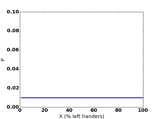
(Yes, I know the value of X is almost certainly not a perfect integer. Let’s simplify and say it is. It doesn’t change the conclusion, I promise. Oh, and I’m also pretending it can’t be 0%. Shhh.)
That’s the probability distribution of X, before we’ve gathered any data. As soon as we start gathering data, it changes.
So we pick a person uniformly at random from Earth, and ask them whether they’re left-handed. They say (in Bengali) that they’re not; they’re right-handed. We can now use some basic probability theory to update X’s distribution to account for this information.
Let A be short for “the person we randomly picked was not left handed”. Then the new distribution
should be P(X|A), meaning “the probability that X has a particular value, given our observation
of a non-left-handed person”. We can compute it like this:
P(X|A) = P(A|X) * P(X)  = (1 - X) * 0.01 = 0.02 (1 - X)
         -------------    --------------
             P(A)              0.5
(The law of probability used in the first step is called Bayes rule.)
So our updated distribution for X—which is called a posterior distribution—is 0.02 (1 - X):
Value of X:   1%     2%     3%  ...   99%  100%
Probability:  2%  1.98%  1.96%  ... 0.02%    0%
As a graph:
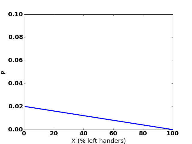
The hypothesis that “literally everyone is left-handed” has been eliminated by the observation of a right-handed person.
If we next see a left-handed person, our distribution for X updates to:
Value of X:      1%     2%  ...  50%  ...   98%    99%
Probability:  0.06%  0.12%  ... 1.5%  ... 0.12%  0.06%
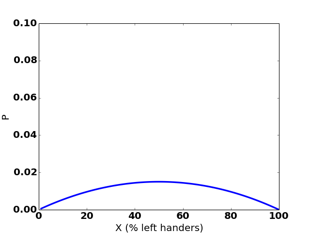
Remember, at this point we’ve seen one leftie and one rightie. So it makes sense that the distribution is symmetric.
Here’s how the graph changes over 35 hypothetical observations:

(The sudden jumps to the right are observations of a left-handed person.)
Say we keep going, and get to 21 lefties out of 243 interviewees (these are the numbers I assumed for Alice’s confidence interval at the beginning of the post). Then our graph will look like this:
Value of X:    1%   2%  ... 5%   6%   7%   8%   9%  10%  11%  12% ...
Probability:  ~0%  ~0%  ... 1%   5%  14%  21%  22%  17%  11%   5% ...
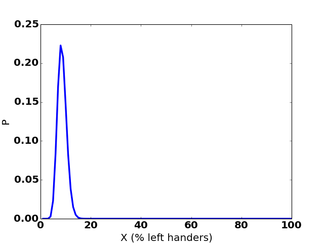
Computing a credible interval from this is easy. The probabilities of the various possibilities for X add up to 100%. The credible interval picks the lower and upper values for X—call them L and U—such that 2.5% of the probability lies below L, 2.5% lies above U, and 95% lies between them. In this case, the credible interval is 5.74% to 12.86%.
So if you accept a uniform prior then there’s a 95% chance that the proportion of the population that is left-handed is between 5.74% and 12.86%.
If you were to pick a different prior, you’d get a different credible interval. There’s an infinite number of possible priors you could pick (and a uniform prior isn’t always appropriate), but every prior leads to exactly one credible interval.
Computing a Confidence Interval
How could you follow in Alice’s footsteps, to compute a confidence interval?
Wikipedia lists five methods for computing a confidence interval for a binomial distribution (i.e., one with a yes/no answer, like “is this person left-handed?”). They are:
- Normal approximation interval
- Wilson score interval
- Jeffry’s interval
- Clopper-Pearson interval
- Agresti-Coull interval
The Normal, Wilson, and Agresti-Coull intervals can be “permissive”, meaning that when you ask for a 95% confidence interval, the probability that the interval contains the true value might be less than 95%. (Personally, I would have called this “wrong”, but “permissive” seems to be the word of art.) So let’s ignore those.
The Clopper-Pearson interval is what I had Alice use. If you ask for a 95% interval, there’s always at least a 95% chance that the interval contains the true value. Though it can be a bit conservative. You can see that in this post: Alice’s confidence interval is a bit wider than the Bayesian credible interval.
The final option is Jeffry’s interval. It is a Baysian credible interval, that also obeys the rules for a confidence interval. As a credible interval, it’s like what we calculated above, except that instead of starting with a uniform distribution, it starts with a beta distribution with parameters (1/2, 1/2). That distribution looks link this, which seems a little odd to me because it says it’s impossible that exactly half of all people might be left-handed.
As a confidence interval, Jeffry’s interval has the bonus property that it’s equally likely for the
true value to lie to either side of the interval. According to Wikipedia, this is in contrast to the
Wilson interval, which is centered too close to X = 1/2.
There’s a lesson here: while the probability that the true value lies outside a randomly generated 95% confidence interval is 5%, the chance it lies above the interval need not be 2.5%.
Conclusion
I think the main takeaways are:
- There is a simple, technical difference between Frequentist and Bayesian interpretations of probability theory: which things in the real world are modeled as constants, and which are modeled as random variables.
- A confidence interval does not tell you how likely it is that the true mean has any particular value. To find out, you must either (i) do Bayesian math, or (ii) reason outside of probability theory.